
ECML-PKDD 2025 · CCF B
SVCT: Stable Vision Concept Transformers for Medical Diagnosis
Official project page
TL;DR
SVCT combines concept-enhanced ViT with denoised diffusion smoothing to retain diagnostic accuracy and produce stable concept-level explanations under perturbations.
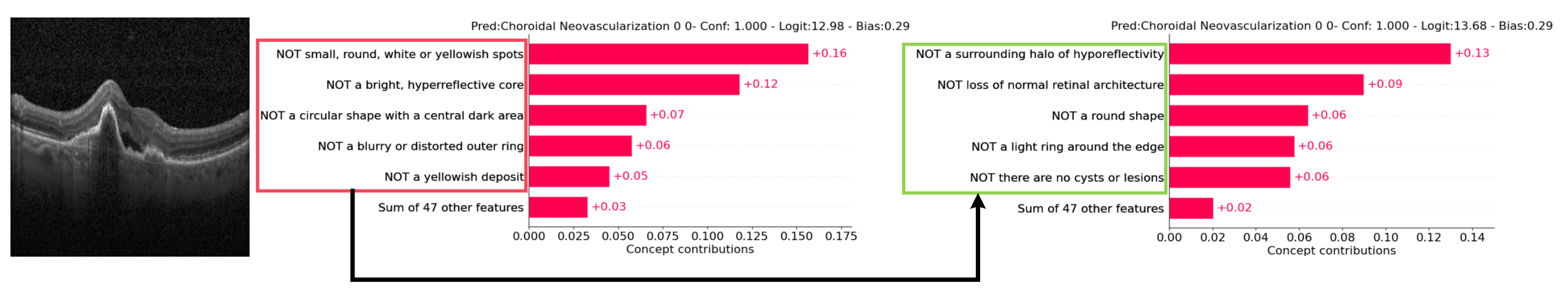
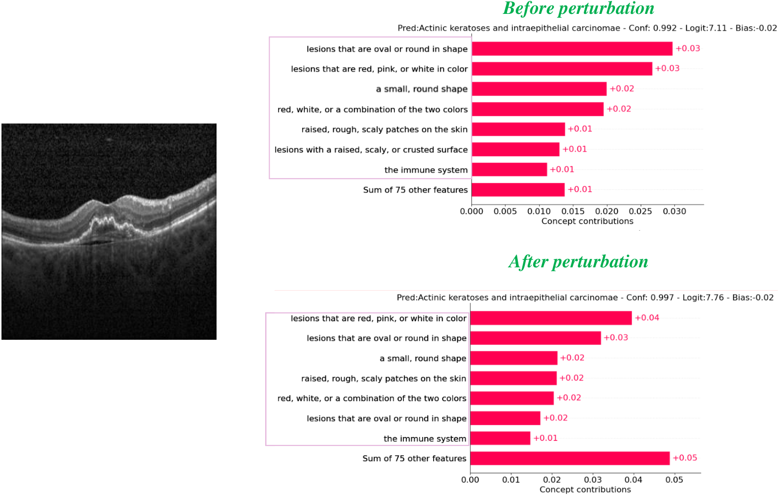
Figure 1: VCT example (OCT2017)
Input image, concept output without perturbation, and concept output after perturbation — illustrating why SVCT is needed for stable explanations.
Abstract
Transparency is a paramount concern in medical AI. Concept Bottleneck Models (CBMs) restrict the latent space to human-understandable concepts, but existing methods often rely solely on concept features for prediction, overlooking intrinsic feature embeddings in medical images, and can be unstable under input perturbations. We propose Vision Concept Transformer (VCT), which uses ViT as the backbone and a label-free conceptual layer, and fuses concept features with image features for decision-making to preserve accuracy while remaining interpretable. We then propose Stable Vision Concept Transformer (SVCT) by integrating Denoised Diffusion Smoothing (DDS) so that the top-k concept indices and predictions remain stable under perturbations, providing faithful explanations. Experiments on four medical datasets (HAM10000, Covid19-CT, BloodMNIST, OCT2017) show that VCT and SVCT maintain accuracy and interpretability, and SVCT provides stable explanations under perturbations.
Figure 2: SVCT framework overview
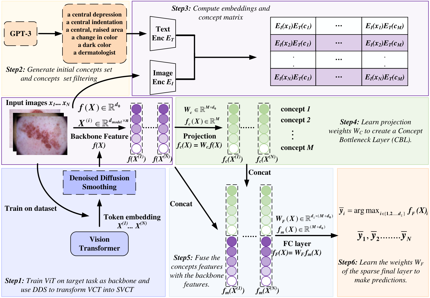
Overview of the Stable Vision Concept Transformer (SVCT) model.
Method: VCT and SVCT
VCT (Vision Concept Transformer)
- ViT backbone plus a Concept Bottleneck Layer learned in a label-free way (e.g. CLIP-Dissect).
- Concept features f_c(X) are fused with backbone features: F(X) = concat(f(X), W_c f(X)) for the final classifier, avoiding the accuracy drop of concept-only CBMs.
SVCT (Stable VCT)
- Apply Denoised Diffusion Smoothing: add Gaussian noise to token embeddings, then denoise with a diffusion model.
- This yields a stable concept module: (i) explanation stability — top-k concept overlap ≥ β under perturbation; (ii) prediction robustness — Rényi divergence between predictions bounded.
- Default noise level σ = 8/255; evaluation uses perturbation radii ρ_u ∈ [6/255, 10/255].
Experiments (from paper)
Datasets: HAM10000, Covid19-CT, BloodMNIST, OCT2017. Perturbation: PGD radius ρ_u ∈ [6/255, 10/255]; DDS noise σ = 8/255.
Accuracy (with/without perturbation)
| Method | HAM10000 | Covid19-CT | BloodMNIST | OCT2017 |
|---|---|---|---|---|
| Standard (No interpretability) | 99.13% | 81.62% | 97.05% | 99.70% |
| Label-Free CBM | 93.61% | 79.75% | 94.97% | 97.50% |
| Post-hoc CBM | 97.60% | 76.26% | 94.83% | 98.60% |
| VCT | 99.00% | 80.62% | 96.21% | 99.10% |
| SVCT | 99.05% | 81.37% | 96.96% | 99.50% |
| ρ_u=8/255 − LF-CBM | 90.08% | 67.98% | 80.53% | 91.88% |
| ρ_u=8/255 − SVCT | 97.97% | 74.45% | 94.07% | 98.70% |
| ρ_u=10/255 − LF-CBM | 88.70% | 65.12% | 75.63% | 90.58% |
| ρ_u=10/255 − SVCT | 97.24% | 71.65% | 92.65% | 98.48% |
Stability: CFS and CPCS
CFS ↓ (lower is better), CPCS ↑ (higher is better). SVCT consistently achieves best stability.
| Method | HAM10000 (CFS/CPCS) | Covid19-CT (CFS/CPCS) | BloodMNIST (CFS/CPCS) | OCT2017 (CFS/CPCS) |
|---|---|---|---|---|
| ρ_u=6/255 − LF-CBM | 0.3335 / 0.9405 | 0.6022 / 0.8117 | 0.5328 / 0.8511 | 0.3798 / 0.9254 |
| ρ_u=6/255 − SVCT | 0.1354 / 0.9900 | 0.5555 / 0.8359 | 0.3589 / 0.9320 | 0.3257 / 0.9468 |
| ρ_u=8/255 − LF-CBM | 0.3719 / 0.9256 | 0.6707 / 0.7710 | 0.6280 / 0.7947 | 0.3941 / 0.9196 |
| ρ_u=8/255 − SVCT | 0.1555 / 0.9867 | 0.6446 / 0.7818 | 0.4383 / 0.8977 | 0.3459 / 0.9387 |
| ρ_u=10/255 − LF-CBM | 0.4027 / 0.9123 | 0.7224 / 0.7336 | 0.6906 / 0.7545 | 0.4055 / 0.9145 |
| ρ_u=10/255 − SVCT | 0.1725 / 0.9836 | 0.7096 / 0.7389 | 0.5058 / 0.8625 | 0.3620 / 0.9321 |
Sensitivity and specificity
| Method | HAM10000 (Sen/Spec) | Covid19-CT (Sen/Spec) | BloodMNIST (Sen/Spec) | OCT2017 (Sen/Spec) |
|---|---|---|---|---|
| Label-free CBM | 0.8878 / 0.9827 | 0.7984 / 0.8608 | 0.9407 / 0.9956 | 0.9750 / 0.9960 |
| SVCT | 0.9899 / 0.9999 | 0.8191 / 0.8037 | 0.9667 / 0.9958 | 0.9950 / 0.9994 |
| ρ_u=10/255 − LF CBM | 0.6779 / 0.9615 | 0.5794 / 0.9810 | 0.5880 / 0.9998 | 0.8380 / 0.9880 |
| ρ_u=10/255 − SVCT | 0.9180 / 0.9932 | 0.7136 / 0.9303 | 0.8681 / 0.9948 | 0.9790 / 0.9923 |
Ablation (DDS)
Both denoising and smoothing are essential. Best accuracy and stability (lowest CFS, highest CPCS) when both are enabled. See paper for full ablation tables.
Model configuration & computational cost
Config (paper Table 4): batch_size 512, saga_batch_size 256, proj_batch_size 5000, clip_cutoff 0.25, proj_steps 1000, interpretability_cutoff 0.45, lam 0.0007, n_iters 1000, ρ_u ∈ [6/255, 10/255], S = 8/255.
Cost: ViT 85.8M params / 17.56 GFLOPS; Label-free CBM 85.76M (+40K); SVCT 85.85M (+43K), same GFLOPS.
Visualizations
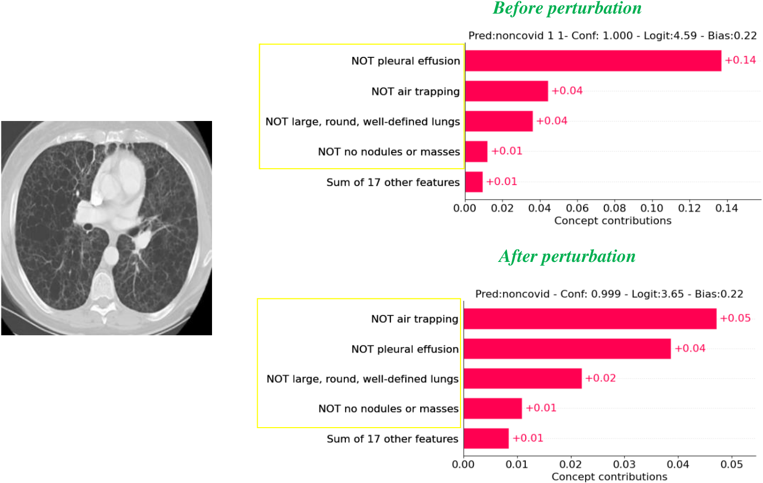
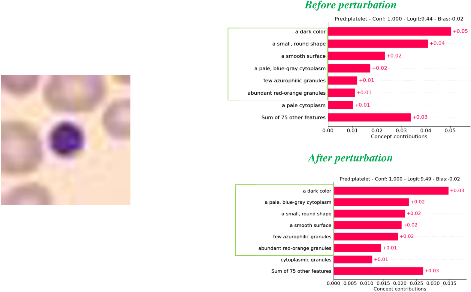
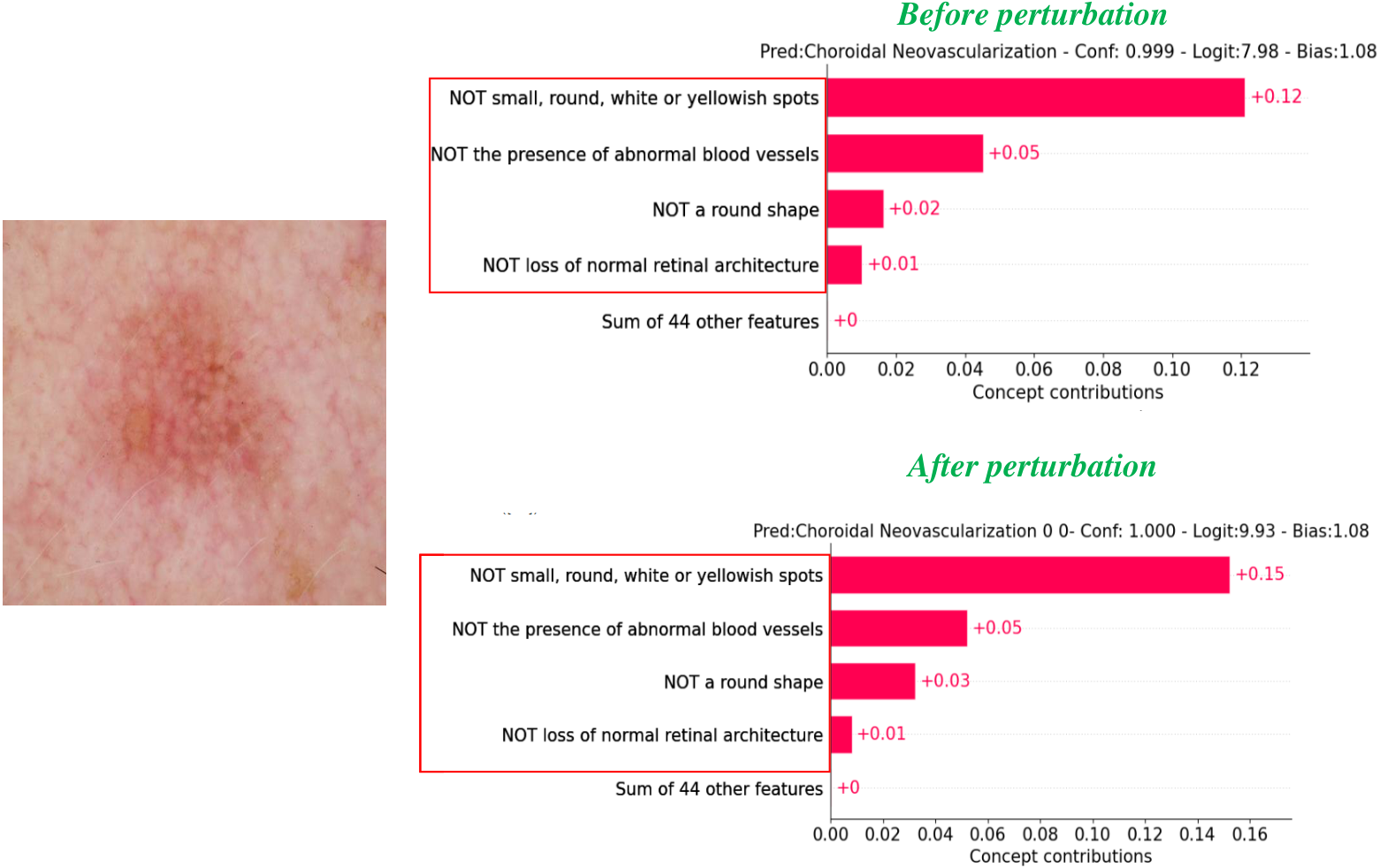
Figure 3: Concept visualization — one sample per dataset, before vs after perturbation.
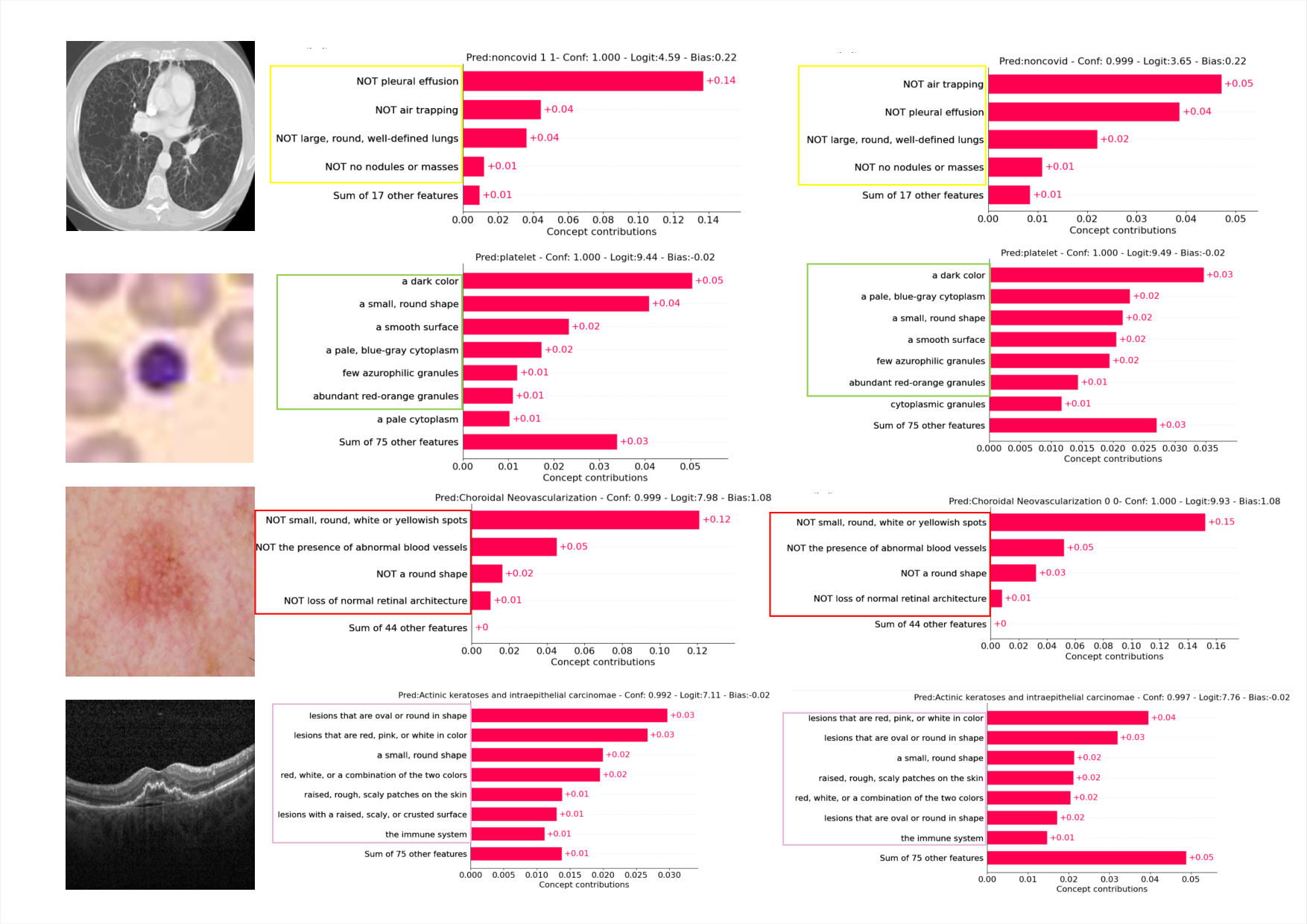
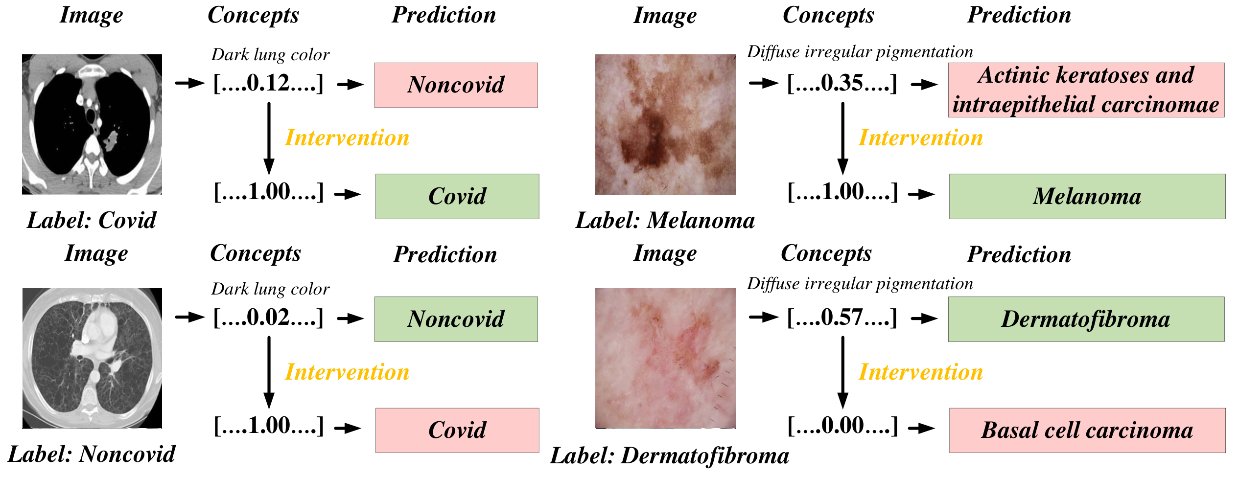
Figure 4: Concept-intervention examples — experts can correct concept predictions for co-diagnosis.
Per-dataset concept weight visualizations (one sample each: Covid19-CT, BloodMNIST, HAM10000, OCT2017).
Code & Repo
- GitHub (code, notebooks, data): github.com/xll0328/-ECML-2025-SVCT
- Paper (PDF): arXiv:2506.05286
Citation
@inproceedings{hu2025stable,
  title     = {Stable Vision Concept Transformers for Medical Diagnosis},
  author    = {Hu, Lijie and Lai, Songning and Hua, Yuan and Yang, Shu and Zhang, Jingfeng and Wang, Di},
  booktitle = {Proceedings of the European Conference on Machine Learning and Principles and Practice of Knowledge Discovery in Databases (ECML-PKDD)},
  year      = {2025}
}