This paper was accepted at ACM MM 2025 (33rd ACM International Conference on Multimedia, October 27–31, 2025, Dublin, Ireland). CCF A, Core A* · Code (GitHub)

Authors: Songning Lai, Ninghui Feng, Jiechao Gao, Hao Wang, Haochen Sui, Xin Zou, Jiayu Yang, Wenshuo Chen, Lijie Hu, Hang Zhao, Xuming Hu, Yutao Yue

Framework (from paper)

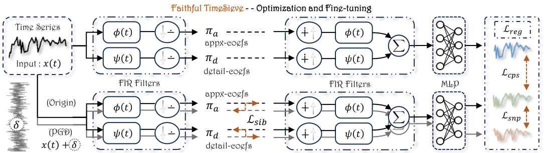
Framework of our proposed Faithful TimeSieve (FTS).

Abstract

The domain of time series forecasting has gained significant attention due to its critical applications in multimedia-rich web traffic (video streaming workloads, dynamic content delivery) and cross-platform advertisement click predictions. While TimeSieve has demonstrated strong capabilities in predicting web visitation metrics, it suffers from critical unfaithfulness issues: sensitivity to random seeds, input noise, layer noise, and parameter perturbations. We propose Faithful TimeSieve (FTS), an enhanced framework that systematically detects and mitigates unfaithfulness in TimeSieve, significantly enhancing its stability and consistency. Experimental results demonstrate that FTS substantially improves the model’s faithfulness and achieves SOTA on multiple datasets, setting a new standard for temporal forecasting methods. This advancement is particularly crucial for web traffic forecasting where prediction accuracy directly impacts operational decisions.

Key Contributions

1. Comprehensive Faithfulness Assessment — In-depth analysis of TimeSieve identifying factors that affect its faithfulness (random seeds, input/layer/parameter perturbations).
2. Definition of Faithful TimeSieve — Rigorous (α₁, α₂, β, δ, R₁, R₂)-Faithful definition with three attributes: Sib, Cps, Snp.
3. Multimedia-aware Robustness Framework — Min-max optimization with PGD and content-adaptive stabilization; framework transfers to other time series models (e.g. PatchTST).
4. Theoretical and Experimental Validation — Bounds for Sib/Cps/Snp and extensive experiments on Wiki, ETTh1, Exchange; FTS achieves SOTA and strong robustness.

Motivation: Why Faithfulness?

• Stability under random seeds — Performance should not vary drastically (e.g. up to ~50% in our study) across different training runs.
• Robustness to input perturbations — Minor input noise led to ~30% performance decline in TimeSieve; FTS recovers via optimization.
• Robustness to layer/parameter perturbations — Model behavior should remain consistent under parameter noise (e.g. IFCB layer).

FTS: Three Attributes (formal)

1. Similarity in IB Space (Sib): Distance D₁ between approximation/detail representations under perturbation is at most β, for all ‖δ‖ ≤ R₁: \(D_1(\hat{\pi}_a(x(t)), \hat{\pi}_a(x(t)+\delta)) \leq \beta \quad \text{(and similarly for } \hat{\pi}_d\text{).}\)
2. Consistency in Prediction Space (Cps): Distance D₂ between predictions under fine-tuned weights and original weights is at most α₁: \(D_2(y(x(t), \tilde{\omega}), y(x(t), \omega)) \leq \alpha_1.\)
3. Stability in Noise Perturbations (Snp): Distance D₃ between predictions under x(t) and x(t)+δ is at most α₂ for all ‖δ‖ ≤ R₂: \(D_3(y(x(t), \tilde{\omega}), y(x(t)+\delta, \tilde{\omega})) \leq \alpha_2.\)

Framework & Loss

The total training objective is:

Here L_reg is the regression loss, L_IB is the TimeSieve IB loss, and L_sib, L_cps, L_snp are the faithfulness auxiliary losses (tied to D₁, D₂, D₃ above). PGD is used to find worst-case perturbation δ, then the fine-tuned weights are updated by gradient descent.

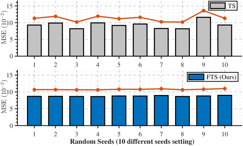
Figure 1: TS vs FTS under 10 random seeds (from paper)

Ten different random seeds are selected to train TimeSieve (TS) and Faithful TimeSieve (FTS) respectively. FTS maintains more consistent performance across seeds.

Main Results

Table 1: Forecasting results (no perturbation)

Forecast length H ∈ {48, 96, 144, 192}, lookback T = 2H. Bold = best, second best.

Table 2: Random seed stability (Exchange, 96-step, MSE)

Baseline seed 2021*. Preference (%) quantifies combined performance and stability (higher = FTS preferred).

Robustness under perturbation (summary)

Under input perturbation (IP) and intermediate-layer perturbation (ILP), FTS with optimization (IPO, ILPO) significantly recovers performance. For example, Wiki 48-step: IP MAE 0.433→0.367 (IPO); ILP MAE 0.453→0.399 (ILPO). See paper for full Table 3.

Loss ablation

Full combination L_total = L_reg + L_IB + λ₁·L_sib + λ₂·L_cps + λ₃·L_snp achieves best. Removing L_snp, L_cps, or L_sib degrades robustness (paper Table 4).

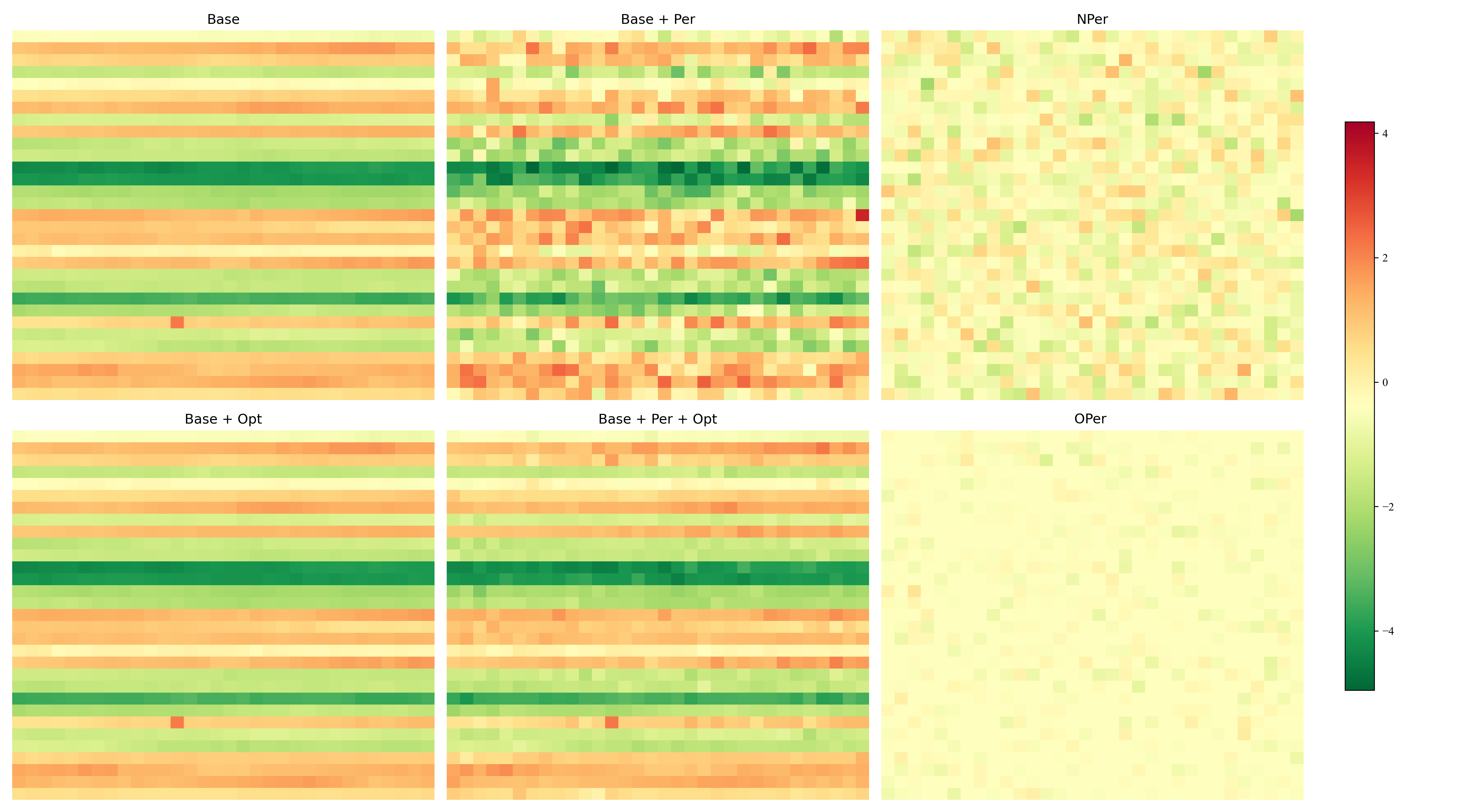
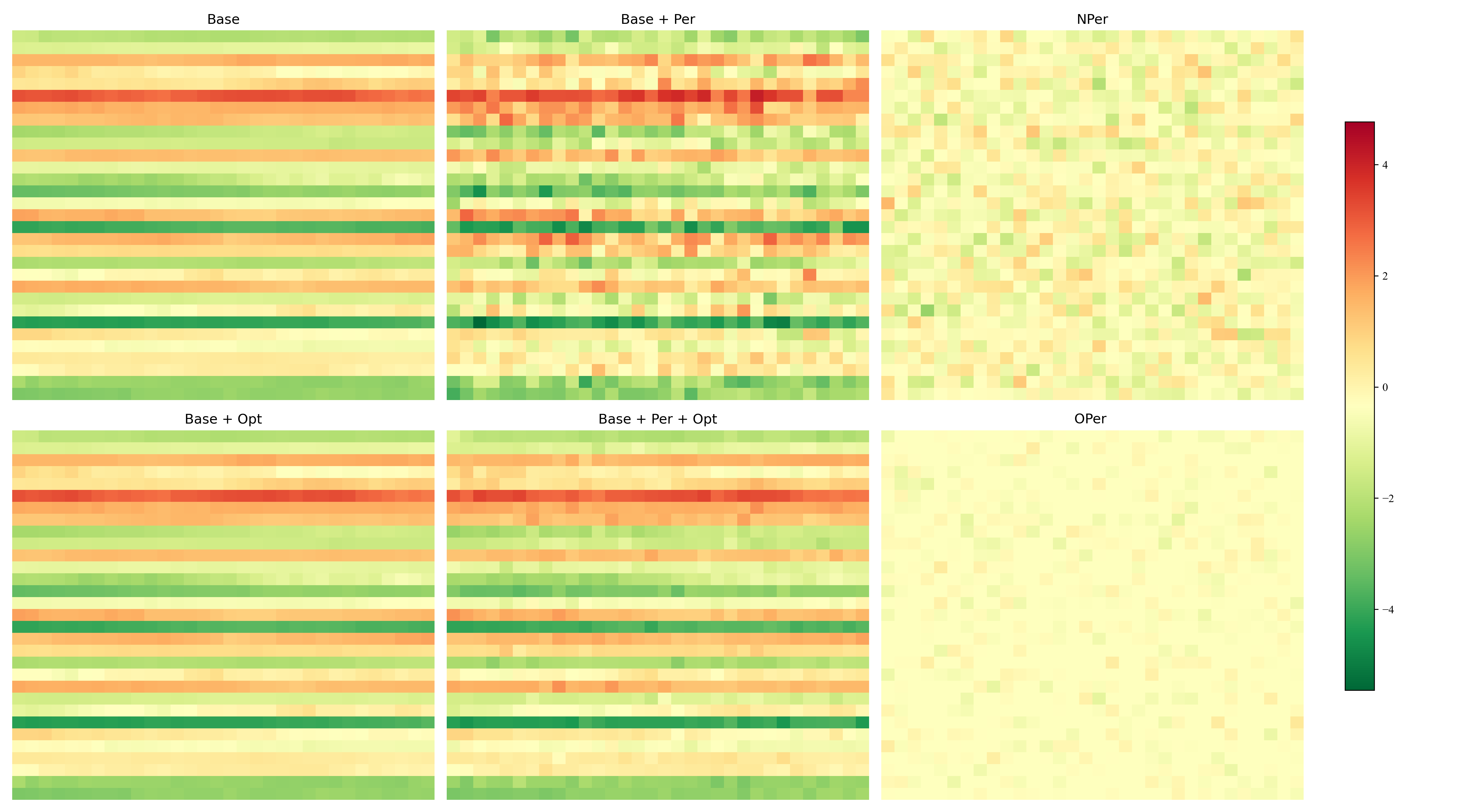
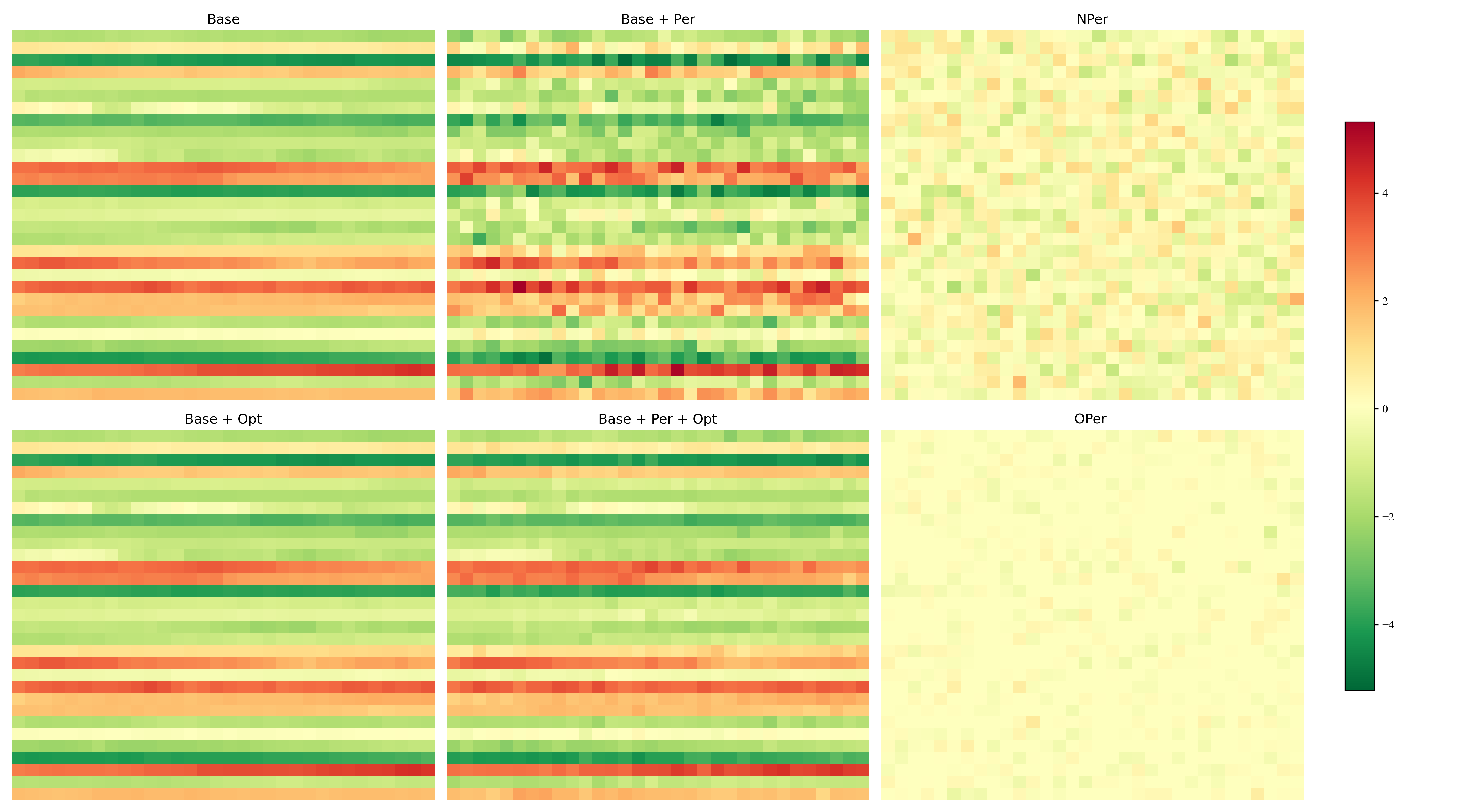
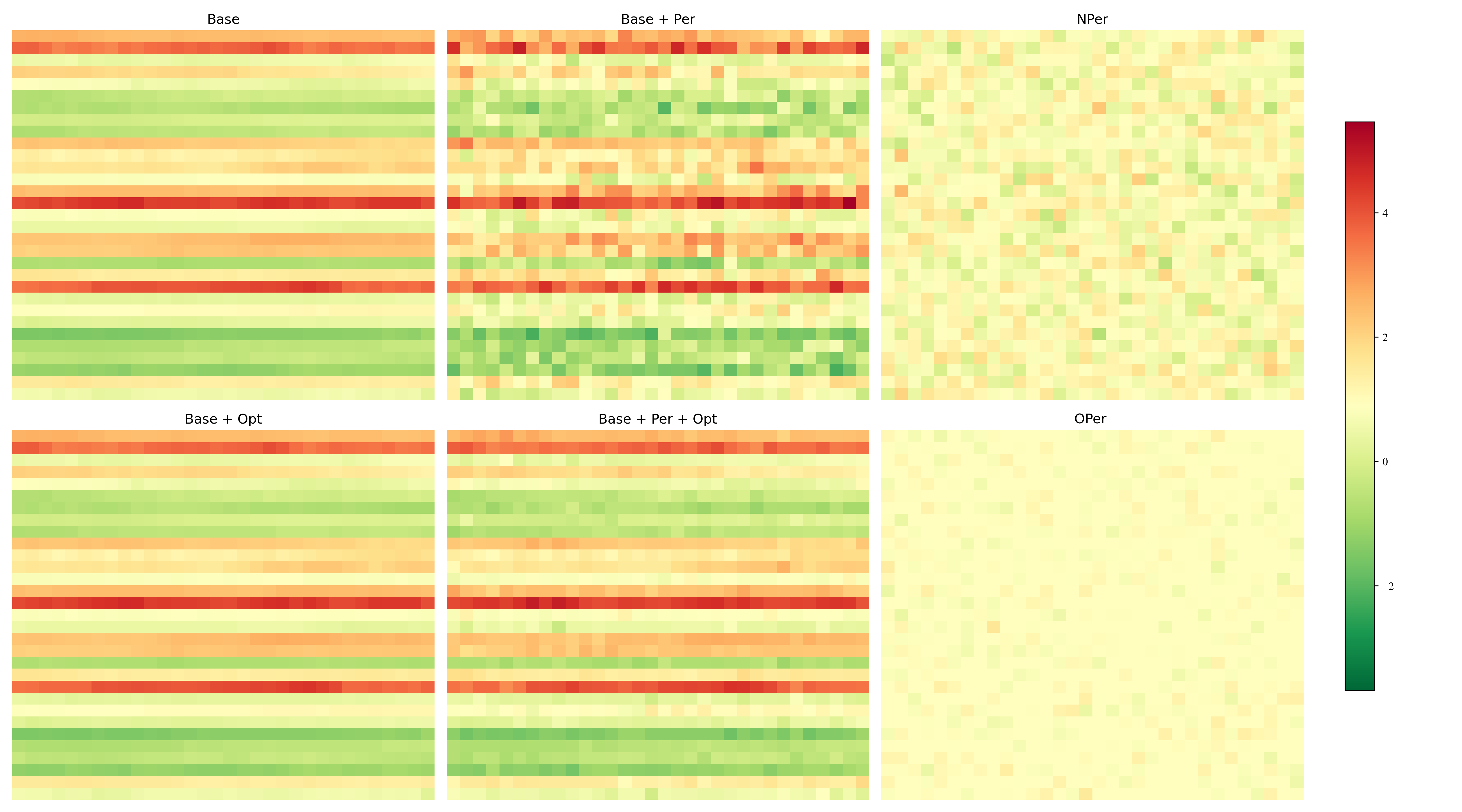
Heatmaps (from paper): prediction length 48, 96, 144, 192

Intermediate layer tensors on Exchange dataset (MSE). Nper vs Oper shows effectiveness of optimization.

Experimental settings (from paper)

• Datasets: Wiki pageviews (top 10 hot words 2015–2016), ETTh1, Exchange.
• Lookback: T = 2H (twice forecast length H).
• Seeds: 10 distinct seeds (2021–2030); 2021 as base.
• Perturbations: Input noise (sequence-decomposition residual); IFCB layer parameter noise (Gaussian).
• Hardware: NVIDIA RTX 4090, Intel Xeon E5-2686 v4. Training: 10 epochs, batch size 32, learning rate 0.0001.

Appendix: Theoretical Derivations

The following presents the proofs for Theorem 1 (upper bound for Sib) and Theorem 2 (lower bound for Sib), and the derivation of the Preference formula used in the main paper.

Theorem 1 (Upper bound for Sib)

Under (α₁, α₂, β, δ, R₁, R₂)-Faithful TimeSieve, for the decoder f: if the distance between IB representations at x(t) and x(t)+δ is at least β (for i ∈ {a, d}), then for all x(t)′ = x(t)+δ with ‖x(t)−x(t)′‖ ≤ R₁,

where the primed representation is at x(t)+δ and c is a constant.

Proof. The approximation and detail coefficients π_a, π_d are defined in the main text (wavelet decomposition). For convenience we omit the argument t. Write

For all ‖δ‖ ≤ R₁,

By normalization of the scaling function, the integral of the scaling function equals 1, so

The same argument applies to π_d. □

Theorem 2 (Lower bound for Sib)

Under (α₁, α₂, β, δ, R₁, R₂)-Faithful TimeSieve, with IB space measured by Rényi divergence D_μ and norm ‖·‖, if δ ∼ N(0, σ²), then for any μ ∈ (1, ∞) and input x(t),

Proof. The Rényi divergence between N(0, σ² I_d) and N(δ, σ² I_d) is bounded by μ‖δ‖²/(2σ²). Thus

When μ R₁²/(2σ²) ≤ β, the FTS framework satisfies Similarity in IB Space (Sib). □

Derivation of Preference Formula

The Preference (%) in the seed-stability table quantifies how much FTS is preferred over TS when changing the random seed. Notation:

• V_ftsb: MSE of FTS under baseline seed (e.g. 2021)
• V_tsb: MSE of TS under baseline seed
• V_ftsc: MSE of FTS under current seed
• V_tsc: MSE of TS under current seed

Step 1 — MSE change:

Step 2 — Ratio of changes:

Step 3 — Adjustment by baseline:

Step 4 — Preference percentage:

Higher preference indicates that FTS is more stable (smaller change when varying the seed) and/or better in MSE relative to TS under the baseline.

Code & Repo

Citation

@inproceedings{lai2025fts,
  title={From Guesswork to Guarantee: Towards Faithful Multimedia Web Forecasting with TimeSieve},
  author={Songning Lai and Ninghui Feng and Jiechao Gao and Hao Wang and Haochen Sui and Xin Zou and Jiayu Yang and Wenshuo Chen and Lijie Hu and Hang Zhao and Xuming Hu and Yutao Yue},
  booktitle={Proceedings of the 33rd ACM International Conference on Multimedia (MM '25)},
  year={2025},
  address={Dublin, Ireland},
}

← Back to Home